Speeding up DQN on PyTorch: how to solve Pong in 30 minutes

Intro

Some time ago I’ve implemented all models from the article Rainbow: Combining Improvements in Deep Reinforcement Learning using PyTorch and my small RL library called PTAN. The code of eight systems is here if you’re curious.

To debug and test it I’ve used Pong game from Atari suite, mostly due to its simplicity, fast convergence, and hyperparameters robustness: you can use from 10 to 100 smaller size of replay buffer and it still will converge nicely. This is extremely helpful for a Deep RL enthusiast without access to the computational resources Google employees have. During implementation and debugging of the code, I was needed to run about 100–200 optimisations, so, it does matter how long one run takes: 2–3 days or just an hour.

Nevertheless you always should keep a balance here: trying to squeeze as much performance as possible, you can introduce bugs, which will dramatically complicate already complex debugging and implementation process. So, after all systems from the rainbow paper were implemented, I asked myself a question: will it be possible to make my implementation faster, to be able to train not only on Pong, but challenge the rest of the games, which require at least 50M frames to train, like SeaQuest, River Raid, Breakout, etc.

As my computational resources are very limited by two 1080Ti + one 1080, (which is very modest nowadays), the only way to proceed is to make the code faster.

Initial numbers

As a starting point, I’ve taken the classical DQN version with the following hyperparameters:

• Environment PongNoFrameskip-v4 from gym 0.9.3 was used,
• Epsilon decays from 1.0 to 0.02 for the first 100k frames, then epsilon kept 0.02,
• Target network synched every 1k frames,
• Simple replay buffer with size 100k was initially prefetched with 10k transitions before training,
• Gamma=0.99,
• Adam with learning rate 1e-4,
• Every training step, one transition from the environment is added to the replay buffer and training is performed on 32 transitions uniformly sampled from the replay buffer,
• Pong is considered solved when the mean score for the last 100 games becomes larger than 18.

The wrappers applied to the environment are very important for both speed and convergence (some time ago I’ve wasted two days of my life trying to find a bug in the working code which refused to converge just because of missing “Fire at reset” wrapper. So, the list of the used wrappers I’ve borrowed from OpenAI baselines project some time ago:

• EpisodicLifeEnv: ends episode at every life lost which helps to converge faster,
• NoopResetEnv: performs random amount of NOOP actions on the reset,
• MaxAndSkipEnv: repeats chosen action for 4 Atai environment frames to speed up training,
• FireResetEnv: presses fire in the beginning. Some environments require this to start the game.
• ProcessFrame84: Frame converted to grayscale and scaled down to 84*84 pixels,
• FrameStack: passes the last 4 frames as observation,
• ClippedRewardWrapper: clips reward to -1..+1 range.

Initial version of code runned on GTX 1080Ti shows the speed of 154 observations per second during training and can solve Pong from 60 to 90 minutes depending on the initial random seed. That’s our starting point.

Convergence dynamics of original version

To put this in perspective, 100M frames which is normally used by RL papers will took us 7.5 days of patient waiting.

Change 1: larger batch size + several steps

The first idea we usually apply to speed up Deep Learning training is larger batch size. It’s applicable to the domain of Deep Reinforcement Learning, but you need to be careful here. In the normal Supervised Learning case, a simple rule “large batch is better” is usually true: you just increase your batch until your GPU memory allows and larger batch normally means more samples will be processed in a unit of time, thanks to the enormous GPU parallelism.

Reinforcement Learning case is slightly different. During the training, two things happen simultaneously:

1. Your network is trained to get better predictions on current data,
2. Your agent is exploring the environment.

As an agent explores the environment and learns about the outcome of its actions, the training data is changing. For example, in a shooter your agent can run randomly for a while beeing shot by monsters, having only miserable “death is everywhere” experience in the training buffer. But after a while, the agent can discover that he has a weapon it can use. This new experience can dramatically change the data we’re using for training.

RL convergence usually lays on fragile balance between training and exploration. If we just increase a batch size without tweaking other options we can easily overfit to the current data (for our shooter example above, your agent can start thinking that “die young” is the only option to minimize suffering and can never discover the gun it has).

So, in 02_play_steps.py we do several steps every training loop and use batch sizes multiplied by this number of steps. But we need to be careful with this number of steps parameter. More steps mean a larger batch size, which should lead to faster training, but at the same time doing lots of steps between training can populate our buffer with samples obtained from the old network.

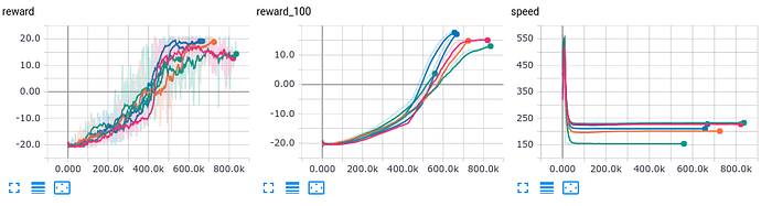
To find a sweet spot, I’ve fixed the training process with a random seed (which you need to pass both numpy and pytorch) and trained it for various steps.

• steps=1: speed 154 f/s (obviously, it’s the same as the original version)
• steps=2: speed 200 f/s (+30%)
• steps=3: speed 212 f/s (+37%)
• steps=4: speed 227 f/s (+47%)
• steps=5: speed 228 f/s (+48%)
• steps=6: speed 232 f/s (+50%)

The convergence dynamics is almost the same (see image below ), but speed the increase saturates around 4 steps, so, I’ve decided to stick to this number for further experiments.

Runs with steps varying from 1 to 6

Ok, we’ve got +47% performance increase.

Change 2: play and train in separate processes

In this step we’re going to check our training loop, which basically contains repetition of the following steps:

1. play N steps in the environment using the current network to choose actions,
2. put observations from those steps into replay buffer,
3. randomly sample batch from replay buffer,
4. train on this batch.

The purpose of the first two steps is to populate the replay buffer with samples from the environment (which are observation, action, reward and next observation). The last two steps are training our network.

The illustration of the above steps and their communication with the environment, DQN on GPU and replay buffer is on the diagram below.

Serial version

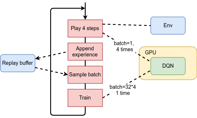
As we can see, the environment is being used only by the first step and the only connection between top and bottom halves of our training is our replay buffer. Due to this data independence, we can run both processes in parallel:

• the first one will communicate with the environment, feeding the replay buffer with fresh data,
• the second will sample training batch from the replay buffer and perform training.

Both activities should run in sync, to keep training/exploration balance we’ve discussed in the previous section.

This idea was implemented in 03_parallel.py and is using torch.multiprocessing module to parallelize playing and training still being able to work with GPU concurrently. To minimize the modifications in other classes, only the first step (environment communication) was put in separate process. The obtained observations were transferred to the training loop using the Queue class.

Parallel version

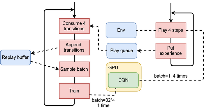
Benchmarking of this new version shows impressive 395 frames/s, which is 74% increase versus the previous version and 156% increase in comparison to the original version of the code.

Change 3: async cuda transfers

The next step is simple: every time we call cuda() method of Tensor we pass async=True argument, which disables waiting for transfer to complete. It won’t give you very impressive speed up, but sometimes gives you something and very simple to implement.

This version is in file 04_cuda_async.py and the only difference is passing cuda_async=True to calc_loss function.

After benchmarking I’ve got 406 frames/s training speed, which is 3.5% speed up to the previous step and 165% increase versus the original DQN.

Change 4: latest Atari wrappers

As I’ve said before, original version of DQN used some old Atari wrappers from OpenAI baselines project. Several days ago those wrappers were changed with commit named “change atari preprocessing to use faster opencv”, which is definetely worth to try.

Here is the new code of the wrappers in the baselines repo. Next version of the DQN is in 05_new_wrapper.py. As I haven’t pulled new wrappers into ptan library, they are in the separate lib in examples.

Benchmarking result is 484 frames/s, which is 18% increase to the previous step and final 214% gain to the original version.

Summary

Thanks for reading!

With several not very complicated tricks we’ve got more than 3 times increase in speed of DQN, without sacrificing readability and adding extra complexity to the code (the training loop is still less than 100 lines of python code). And now, the latest version is able to reach 18 score in Pong in 20–30 minutes, which opens lots of new possibilities to experiment with other Atari games, as 484 frames per second means less than 2.5 days to process 100M observations.

If you know more things that can increase performance of PyTorch code, please leave comments, I am really interested to know them.